Equivariance and Symmetry behind Neural Networks

How symmetry powers the success of convolutional neural networks.

I spent much of the last fall studying abstract algebra, which I find to be one of the most beautiful branches of mathematics. Recently, I had been meditating on the connections between algebra and deep learning, and converged on various ideas in symmetry and equivariance. Below is a concise narrative of some of my learnings on the matter.

What is Symmetry, Really?

To build intuition before diving into formal definitions, consider a simple object: a square.

Figure 0: The eight symmetries of a square.

How many ways can you move this square so that it lands back in its original footprint, looking unchanged? You could rotate it by 0°, 90°, 180°, or 270°. You could also flip it across its horizontal, vertical, or two diagonal axes. These eight transformations, four rotations and four reflections, are the symmetries of the square.

What makes this special is that if you perform one transformation and then another, you get a third transformation that is also on our list. For example, rotating 90° and then flipping horizontally is the same as flipping along one of the diagonals.

This collection of symmetries, with its special property that transformations can be combined, isn’t just a curiosity. It’s an example of a deep mathematical structure. To build powerful AI systems that can understand and leverage these symmetries, we need a formal language to describe them. This brings us to the concept of a group.

Algebra Crash Course

Group Axioms

A group is a set of elements, $G$, equipped with a binary operation, $\circ$, that combines any two elements to form a third. For $(G, \circ)$ to be a group, it must satisfy the below axioms:

Closure: $\forall g_{1}, g_{2} \in G$, $g_{1} \circ g_{2} \in G$
There is an identity element: $\exists e \in G$ such that $\forall g \in G$, $e \circ g = g \circ e = g$.
Composition is associative: $\forall g_{1}, g_{2}, g_{3} \in G$, $(g_{1} \circ g_{2}) \circ g_{3} = g_{1} \circ (g_{2} \circ g_{3})$.
Every element has an inverse: $\forall g \in G$, $\exists h \in G$ such that $g \circ h = h \circ g = e$.

Axioms in Action: Dihedral Group

These axioms can seem abstract and somewhat dry on their own. Let’s make them more concrete by revisiting our square example. In abstract algebra, we can describe the entire group of 8 symmetries with just two generators: a rotation, $r$, and a reflection, $f$. All other transformations can be expressed as combinations of these two. This is known as the presentation of the group:

\[D_{4} = \langle r,f | r^4 = e, f^2 = e, rf = fr^{-1} \rangle\]

This compact notation tells us everything we need to know:

$r^4 = e$: rotating four times by 90° is the same as doing nothing (the identity action, $e$).
$f^2 = e$: reflection twice is the same as doing nothing.
$rf = fr^{-1}$: this relation informs us about the interaction between rotations and reflections; notably, this rule makes the group non-abelian (that is, the order of operations matter) ¹.

Using this presentation, the eight elements of the group are:

\[D_{4} = \lbrace e, r, r^2, r^3, f, fr, fr^2, fr^3 \rbrace\]

Here, $r$ represents a 90° rotation, $r^2$ represents a 180° rotation, and so on. $f$ can be any one of the reflections (e.g., a reflection about the vertical axis), and then the other reflections can be generated, such as $fr$ (a 90° rotation followed by reflection about the vertical axis, which is equivalent to reflection about the diagonal from top-left to bottom-right).

This structure is neatly captured in the group’s multiplication table, or Cayley table. The operation is composition (apply the row element, then the column element).

$\circ$	$e$	$r$	$r^2$	$r^3$	$f$	$fr$	$fr^2$	$fr^3$
$e$	$e$	$r$	$r^2$	$r^3$	$f$	$fr$	$fr^2$	$fr^3$
$r$	$r$	$r^2$	$r^3$	$e$	$fr^3$	$f$	$fr$	$fr^2$
$r^2$	$r^2$	$r^3$	$e$	$r$	$fr^2$	$fr^3$	$f$	$fr$
$r^3$	$r^3$	$e$	$r$	$r^2$	$fr$	$fr^2$	$fr^3$	$f$
$f$	$f$	$fr$	$fr^2$	$fr^3$	$e$	$r$	$r^2$	$r^3$
$fr$	$fr$	$fr^2$	$fr^3$	$f$	$r^3$	$e$	$r$	$r^2$
$fr^2$	$fr^2$	$fr^3$	$f$	$fr$	$r^2$	$r^3$	$e$	$r$
$fr^3$	$fr^3$	$f$	$fr$	$fr^2$	$r$	$r^2$	$r^3$	$e$

This table provides everything we need to quickly verify that $D_4$ is indeed a group.

Closure: Every cell inside the table contains an element from our original set of eight: $e, r, r^2, r^3, f, fr, fr^2, fr^3$. No new elements are created by composition, so the group is closed.
Identity: The first row and first column, corresponding to composition with the identity element $e$, are identical to the group’s headers. This shows that $e \circ g = g = g \circ e$ for any element $g$.
Associativity: As the elements of $D_4$ are symmetries (bijections of the square), their composition behaves like function composition – which is always associative.
Inverses: From the presentation, we can explicitly construct inverses: $r^k$ has inverse $r^{4-k}$ (as $r^k \circ r^{4-k} = r^4 = e$) and $fr^k$ has inverse $fr^{k}$ as $(fr^k)(fr^{k}) = (r^{-k} f) fr^{k} = r^{-k} e r^k = e$.

Group Actions

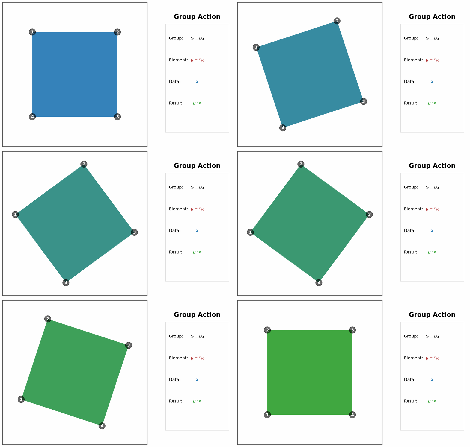
As we have seen, a group is an abstract structure of transformations, but we can truly see the application of this theory when it acts upon data. The concept of group actions is the crucial link between the algebra of symmetries and the world of images, graphs, or sounds that our neural network process. A group action is a formal rule that describes how each element of a group predictably transforms an object.

Rather than starting with the formal definitions, take a look at the following animation.

**Figure 1: A Visual of a Group Action.** The group element $g$ (a 90° rotation) from the group $D_4$ acts on the data $x$ (the initial square) to produce the transformed data $g \cdot x$.

With this visual intuition, the formal definition becomes clearer. A group $G$ acts on a data space $X$ if there is a mapping that takes a group element $g \in G$ and a data point $x \in X$ and gives us a new data point $g \cdot x$. This mapping must respect the group’s structure through two simple axioms:

Identity: The identity element $e \in G$ leaves the data unchanged ($e \cdot x = x$ for all $x \in X$). In our example, if we had used the $e \in D_4$ element (which corresponds to a rotation by 0°), the square would have remained in its original blue state.
Compatibility: Applying two transformations in sequence is the same as applying their single, combined transformation. Formally, $h \cdot (g \cdot x) = (h \circ g) \cdot x$ for all $g, h \in G$ and all $x \in X$.

Equivariance and Invariance

Now that we understand how a group action transforms data, we can ask a critical question: how should a function, like a neural network layer, behave when its input is transformed? This brings us to the core concepts of equivariance and invariance.

Equivariance: The Transformation Commutes with the Function

A function is equivariant if it doesn’t matter whether we transform the input first and then apply the function, or apply the function first and then transform the output. The transformation and the function “commute.”

Let’s make this concrete with our square example. Imagine a function $\mathcal{F}$ that “detects the corner labeled 1.” The figure below shows what happens when we combine this function with our $r_{90}$ rotation.

Since both paths produce the identical final output, the function $\mathcal{F}$ is equivariant to the rotation group. The corner detector’s output rotates just as the input image rotates.

**Figure 2: A Visual Walkthrough of Equivariance.** Following two different paths—(1) rotating then detecting the corner, versus (2) detecting the corner then rotating the result—yields the exact same output. The corner detection is therefore equivariant to rotation.

Formally, let $\mathcal{F} : X \to Y$ be a function that maps from an input data space $X$ to an output space $Y$ (e.g., a feature map). Assume a group $G$ acts on both $X$ and $Y$. Then, $\mathcal{F}$ is equivariant if:

\[\mathcal{F} (g \cdot x) = g \cdot \mathcal{F}(x) \quad \forall g\in G, x \in X\]

This property is crucial for the intermediate layers of a CNN, ensuring that feature detection (like finding edges or textures) is consistent across all locations in an image.

Formal Definition of Invariance

Invariance is a stricter, simpler case of equivariance. A function is invariant if its output is completely insensitive to transformations of the input.

Imagine a different function, $\mathcal{F}_{\text{class}}$, whose job is to “classify the shape.” If we feed it the original blue square, the output is "square", and if we feed it the rotated green square, the output is still "square".

Formally, $\mathcal{F}$ is invariant if:

\[\mathcal{F}(g \cdot x) = \mathcal{F}(x) \quad \forall g \in G, x \in X\]

This is the desired property for a final classification layer. The label of an object should not change just because it has been shifted, rotated, or otherwise transformed.

Convolutional Neural Networks

Convolutional Neural Networks (CNNs) are a class of neural networks that have become the de facto standard for computer vision tasks. Their architecture is specifically designed to process data with a grid-like topology, such as an image. The core building block of a CNN is the convolution layer. Contrasting with traditional neural networks which consist of dense connections, a convolution layer uses a set of learnable filters, or kernels. Each filter is a small matrix of weights that slides – or convolves – across the input image, detecting specific local features like edges, corners, or textures. As the filter moves, it produces a feature map that highlights where these patterns occur in the image. This is typically followed by a pooling layer, such as max-pooling, which downsamples the feature map to make the representation more manageable and robust.

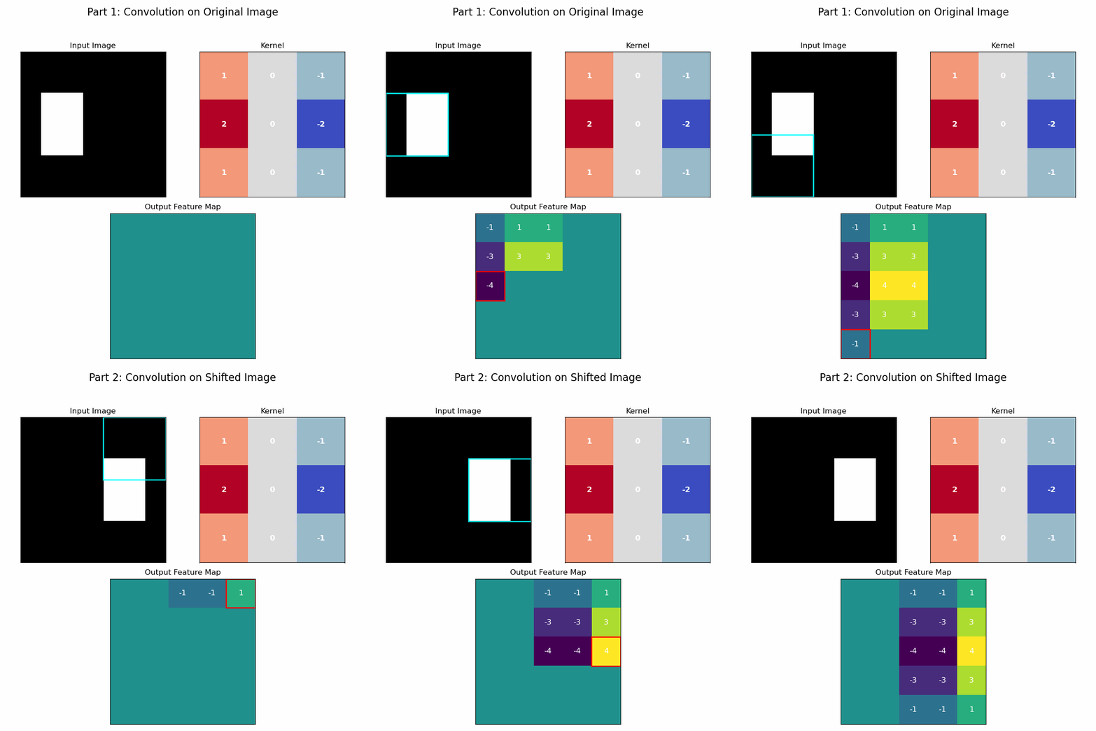
The reason this architecture is so remarkably effective brings us back to the principles of symmetry. The convolution operation, with its sliding filter and shared weights, is a direct, practical implementation of translational equivariance. This translational symmetry itself forms a group, as it satisfies the axioms: combining two shifts results in a net shift (closure), a zero-pixel shift is the identity, every shift has an inverse (shifting back), and the order of shifts is associative. Because the same filter is applied across all spatial locations, if a feature in the input image shifts, its representation in the feature map will shift by the exact same amount.

The animation below brings this to life. In the first half, a filter convolves over an image to produce a feature map. In the second half, the input image is shifted, but the exact same filter is applied. As you can see, the resulting feature map is identical to the first, merely shifted.

**Figure 3: A Demonstration of Translational Equivariance.** The same filter is applied to an image and its shifted version. Notice how the output activation map for the shifted input is an identical, but shifted, version of the original's output.

The Role of Pooling

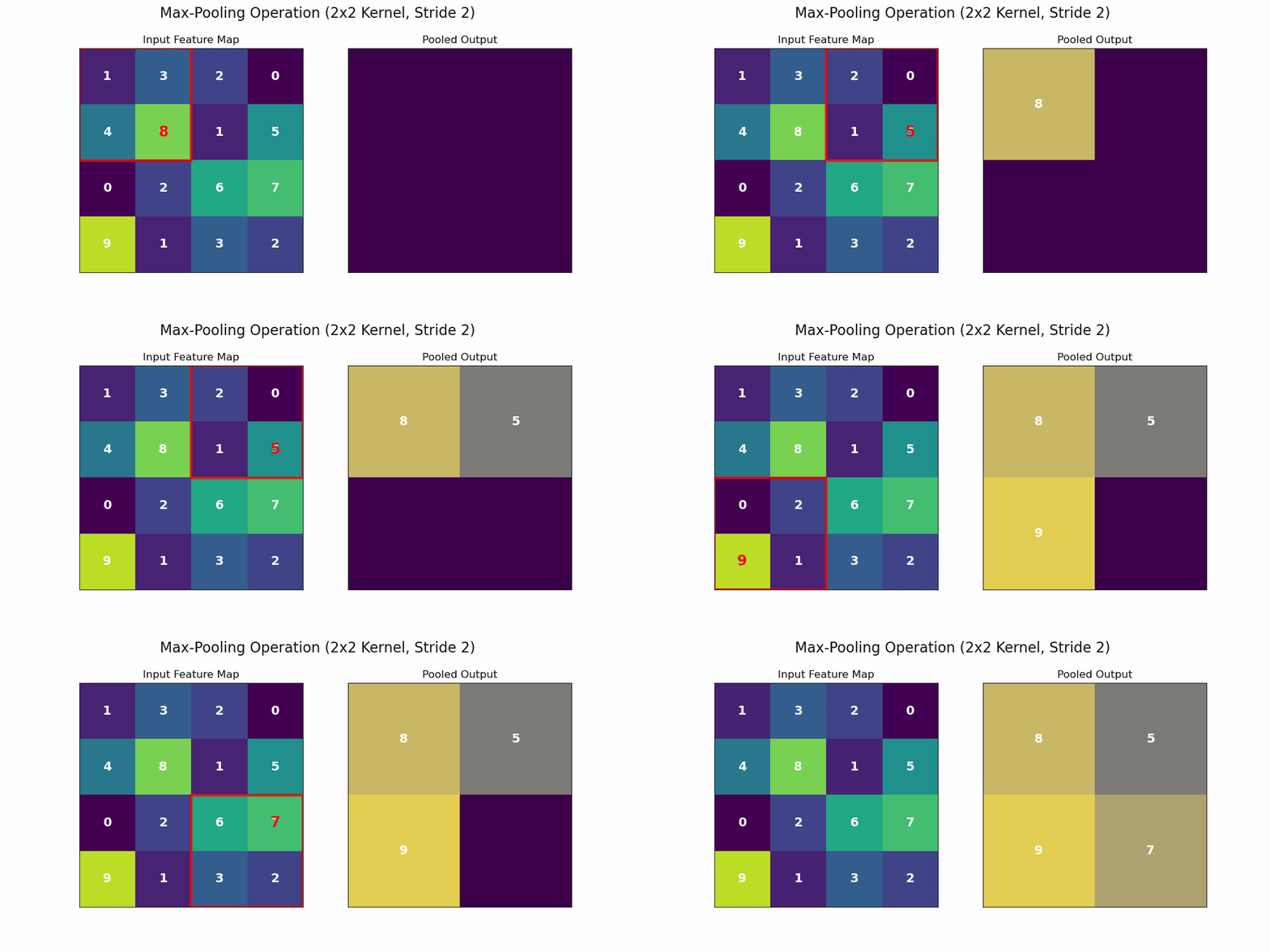
An important caveat is that for a final classification, we often desire invariance – that is, the final label should not change at all if an object’s position shifts slightly. The pooling layer is a key step towards this goal.

By summarizing a local neighborhood with a single value (e.g., the maximum), the network becomes less sensitive to the precise location of features. The animation above shows a max-pooling layer in action. Even if a feature’s activation shifts slightly within a quadrant, as long as it remains the maximum value in that local region, the output of the pooling layer will be identical. This process of composing equivariant convolutional layers with locally invariant pooling layers allows the network to build a representation that is both rich in features and robust to their exact spatial location.

**Figure 4: A Demonstration of Local Invariance from Max-Pooling.** The 2x2 pooling window slides across the feature map, selecting only the maximum value from each quadrant.

It is this hierarchical composition that gives a deep CNN its power. The first convolutional layer finds simple patterns like edges. The subsequent pooling layer makes the representation locally invariant to the exact position of those edges. The next convolutional layer then learns to combine these edge features into more complex patterns, like corners or textures. The next pooling layer makes those features locally invariant. This process repeats, building a representation that is progressively more abstract and robust to transformations, until the final layers can perform a fully invariant classification.

Broadening the Scope

The principles of symmetry and equivariance are not confined to the translational symmetry of images. In fact, they form a foundational design pattern across many of modern deep learning’s most powerful architectures.

Graph Neural Networks (GNNs): Graphs possess a different kind of symmetry: permutation symmetry. The structure of a graph is defined by its nodes and their connections, not by the arbitrary order in which they might be listed in an adjacency matrix. GNNs are designed to respect this by using a message-passing mechanism, where a node’s representation is updated by aggregating information from its neighbors. This aggregation is order-independent, making the GNN permutation equivariant. If you permute the nodes in the input, the output node embeddings are simply permuted in the exact same way.
Transformers: The self-attention mechanism at the heart of the Transformer architecture is also fundamentally permutation equivariant. It treats the input sequence as a set of tokens, evaluating the interaction of every token with every other token, irrespective of their initial positions. This is precisely why positional encodings must be explicitly added to the input embeddings. Without them, the Transformer would be unable to distinguish between “the cat sat on the mat” and “the mat sat on the cat.” This provides a fascinating contrast to CNNs, where geometric structure is a built-in feature rather than an additive one.

Conclusion - The Power of Inductive Bias

We began with the formal, abstract language of group theory and arrived at the practical success of modern neural networks. The connection is a profound one: the most effective architectures are often those that intentionally embody the intrinsic symmetries of their data.²

By building models like CNNs to be equivariant to translation, we provide them with a powerful inductive bias. The model does not need to waste its learning capacity discovering the fundamental rule that an object’s identity is independent of its location; this knowledge is hard-coded into its architecture. This has two critical benefits: (1) Data Efficiency, that is the model can learn from far fewer examples because it automatically generalizes its knowledge across all possible translated positions; and (2) Better Generalization, that is the model is more robust and performs better on unseen data because it is founded on a more fundamental understanding of the data’s structure.

These ideas – of identifying the underlying symmetry of a domain and constructing equivariant models – are the cornerstone of Geometric Deep Learning. This approach suggests the path to more capable AI may lie not just in bigger datasets, but in building models that perceive the world through the elegant and powerful lens of symmetry.

Acknowledgements

I would like to extend my heartfelt thanks to my friends for their insightful discussions and for proofreading early drafts of this article. Their feedback was invaluable in refining the narrative.

Special thanks are also due to Nick James, whose critical feedback prompted a significant revision of the introductory sections. His push for more geometric intuition and visual examples, specifically referencing the dihedral group and the value of visual group theory, greatly improved the final result.